END-TO-END PIPELINE
Purpose of the notebook
This notebook includes an end-to-end pipeline prepared to run a detailed analysis of Xenium samples. It includes tasks such as: 1. Formatting xenium output to AnnData files, filtering reads by distance to nuclei or quality 2. Resegmenting cells using Baysor (using Docker/Singularity) 3. Preprocessing and clustering cells in the experiment, generating spatial maps and differentially expressed genes 4. Imputing gene expression using SpaGE 5. Domain identification using Banksy(preferred) ,neighbor-based domains or read-based domains 6. Identifying Spatially variable genes using Squidpy’s Moran’s I 7. Defining celltype neighborhood enrichment using Squidpy
Import packages
[58]:
import os
import numpy as np
import pandas as pd
import scanpy as sc
import seaborn as sns
import matplotlib.pyplot as plt
from xb.formatting import *
from xb.plotting import *
from xb.preprocessing import *
from xb.Spage_main import *
from xb.calculating import *
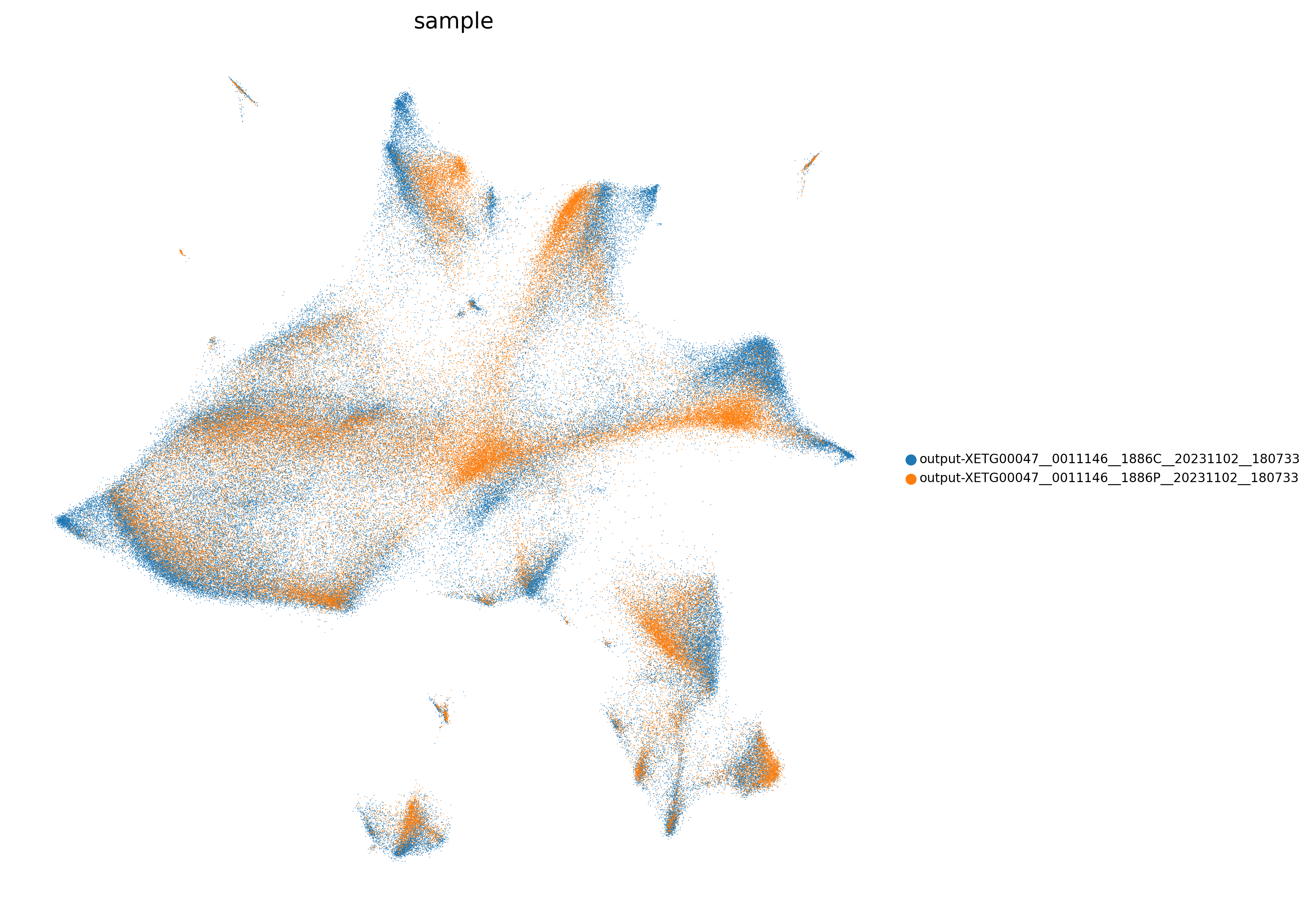
0. Defining input parameters
We first define some basic information for our path including: - Files: list including the paths where your Xenium output is stored for each experiment - Output_path: directory where you want to save the ouptut of your pipeline - save: whether you want to save intermediate files and plots - plot_path: path to the directory where figures generated should be saved, if applicable
OBS! Downloading example dataset: For downloading Xenium example dataset, please use the following link: https://doi.org/10.5281/zenodo.11612060 and include the path of the downloaded files under files
[5]:
files=['./data/data_end_to_end_pipeline/output-XETG00047__0011146__1886C__20231102__180733',
      './data/data_end_to_end_pipeline/output-XETG00047__0011146__1886P__20231102__180733']
output_path=r'../pipeline_output/'
save=True ## Saving intermediate outputs
plot_path=output_path+'/figures/'
1. Format Xenium output to AnnData
First, we will format the Xenium datasets to AnnData format, filtering in the process reads that have either too low quality or that are too far away from the segmented cell body. Fo this we need to define two parameters: - Max_nucleus_distance: maximum distance from the reads to each closest cell to consider reads in the definition of cells - min_quality: minimum quality of reads to be kept in the analysis
[3]:
max_nucleus_distance=10
min_quality=0
Now we run the function format_to_adata to format Xenium’s output to AnnData
[6]:
adata=format_to_adata(files=files,output_path=output_path,max_nucleus_distance=max_nucleus_distance,min_quality=min_quality,save=save)
Formatting output-XETG00047__0011146__1886C__20231102__180733
/media/sergio/xenium_b_and_heart/actual_repo/Xenium_benchmarking/xb/formatting.py:536: FutureWarning: X.dtype being converted to np.float32 from int64. In the next version of anndata (0.9) conversion will not be automatic. Pass dtype explicitly to avoid this warning. Pass `AnnData(X, dtype=X.dtype, ...)` to get the future behavour.
  adata=sc.AnnData(ad.transpose(),obs=cell_info,var=features)
/home/sergio/anaconda3/envs/xb_dev3/lib/python3.7/site-packages/anndata/_core/anndata.py:121: ImplicitModificationWarning: Transforming to str index.
  warnings.warn("Transforming to str index.", ImplicitModificationWarning)
Filter reads
/media/sergio/xenium_b_and_heart/actual_repo/Xenium_benchmarking/xb/formatting.py:628: FutureWarning: X.dtype being converted to np.float32 from int64. In the next version of anndata (0.9) conversion will not be automatic. Pass dtype explicitly to avoid this warning. Pass `AnnData(X, dtype=X.dtype, ...)` to get the future behavour.
  adata1nuc=sc.AnnData(np.array(ct1),obs=adataobs,var=av)
Formatting output-XETG00047__0011146__1886P__20231102__180733
/media/sergio/xenium_b_and_heart/actual_repo/Xenium_benchmarking/xb/formatting.py:536: FutureWarning: X.dtype being converted to np.float32 from int64. In the next version of anndata (0.9) conversion will not be automatic. Pass dtype explicitly to avoid this warning. Pass `AnnData(X, dtype=X.dtype, ...)` to get the future behavour.
  adata=sc.AnnData(ad.transpose(),obs=cell_info,var=features)
/home/sergio/anaconda3/envs/xb_dev3/lib/python3.7/site-packages/anndata/_core/anndata.py:121: ImplicitModificationWarning: Transforming to str index.
  warnings.warn("Transforming to str index.", ImplicitModificationWarning)
Filter reads
/media/sergio/xenium_b_and_heart/actual_repo/Xenium_benchmarking/xb/formatting.py:628: FutureWarning: X.dtype being converted to np.float32 from int64. In the next version of anndata (0.9) conversion will not be automatic. Pass dtype explicitly to avoid this warning. Pass `AnnData(X, dtype=X.dtype, ...)` to get the future behavour.
  adata1nuc=sc.AnnData(np.array(ct1),obs=adataobs,var=av)
/home/sergio/anaconda3/envs/xb_dev3/lib/python3.7/site-packages/anndata/_core/anndata.py:1828: UserWarning: Observation names are not unique. To make them unique, call `.obs_names_make_unique`.
  utils.warn_names_duplicates("obs")
2. Resegmentation using Baysor (Alternative to #1)
Alternatively to define cells based on Xenium’s segmentation, we can also perform Baysor, which we observed to perform slightly better in terms of number of assigned transcripts. For this, we first pormat the Xenium’s to get the input needed for baysor
Note that we also have this functionk in a batch for for multiple inputs. It’s called batch_prep_xenium_data_for_baysor and accepts a list of xenium outputs, stored in files as an input. However, it doesn’t accept to process a crop.
[4]:
prep_xenium_data_for_baysor(files[0], output_path,CROP=True, COORDS=[1000, 5000, 1000, 5000])
CHECKPOINT 1: Output directory created
CHECKPOINT 2: Spots loaded
CHECKPOINT 3: Spots converted to pixel units
CHECKPOINT 4: Spots cropped
CHECKPOINT 5: Polygons loaded
CHECKPOINT 6: Polygons cropped
CHECKPOINT 7: Label image created
CHECKPOINT 8: Spots saved
CHECKPOINT 9: Polygons saved
CHECKPOINT 10: Label image saved
Next, we will perform Baysor. Since Baysor is implemented in Julia and has its own required environment, we will run it using Docker. First we get the docker we need. Please remember to install docker before if required (https://docs.docker.com/get-docker/). Please run this part from the command line if needed. IMPORTANT We recommend to run this part directly in your command line in case you need to run it as a superuser (with sudo)
[5]:
!docker pull louisk92/txsim_baysor:v0.6.2bin
[sudo] password for sergio:
After that we run the docker container, and within it we run baysor. IMPORTANT We recommend to run this part directly in your command line in case you need to run it as a superuser (with sudo)
[ ]:
# we first run the docker, specifying the path tto the baysor input/output after the fist -v and also the path where the main we will use to run baysor is stored
!sudo docker run -it --rm -v /media/sergio/xenium_b_and_heart/pipeline_output/output-XETG00045__0011129__1225C__20231116__105020_baysor:/media/sergio/xenium_b_and_heart/pipeline_output/output-XETG00045__0011129__1225C__20231116__105020_baysor -v /media/sergio/xenium_b_and_heart/actual_repo/Xenium_benchmarking/xb:/media/sergio/xenium_b_and_heart/actual_repo/Xenium_benchmarking/xb louisk92/txsim_baysor:v0.6.2bin
# next we change directory to the directory where the run_baysor.sh script is.
!cd /media/sergio/xenium_b_and_heart/actual_repo/Xenium_benchmarking/xb
# finally, we run baysor
!bash run_baysor.sh "/media/sergio/xenium_b_and_heart/pipeline_output/output-XETG00045__0011129__1225C__20231116__105020_baysor"
Finally, we define in path where is the output of baysor stored and we format it to anndata. From here, we can continue to step 3 without major issues
[11]:
patha='/media/sergio/xenium_b_and_heart/pipeline_output/output-XETG00045__0011129__1225C__20231116__105020_baysor'
adata=format_baysor_output_to_adata(path,output_path)
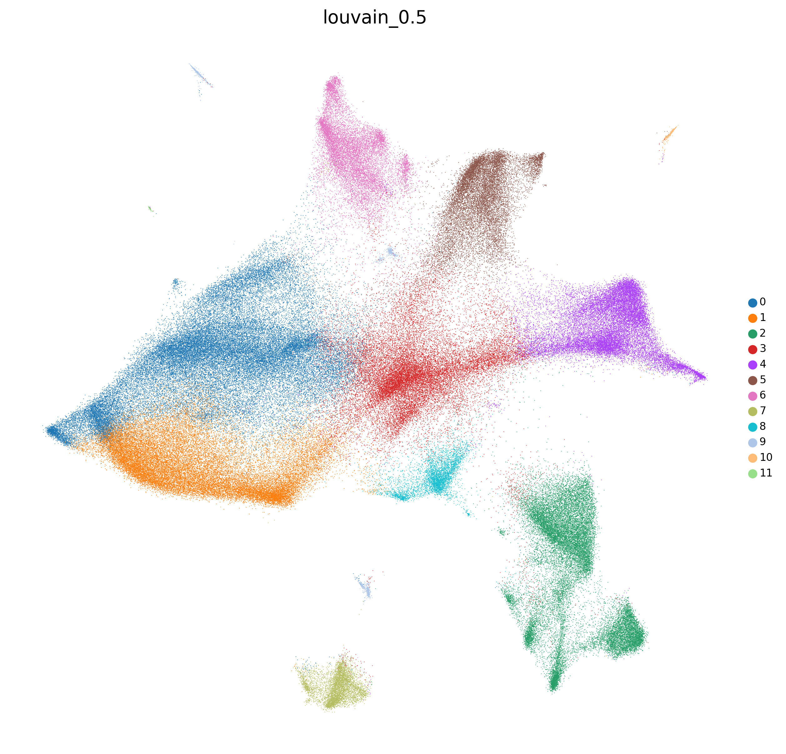
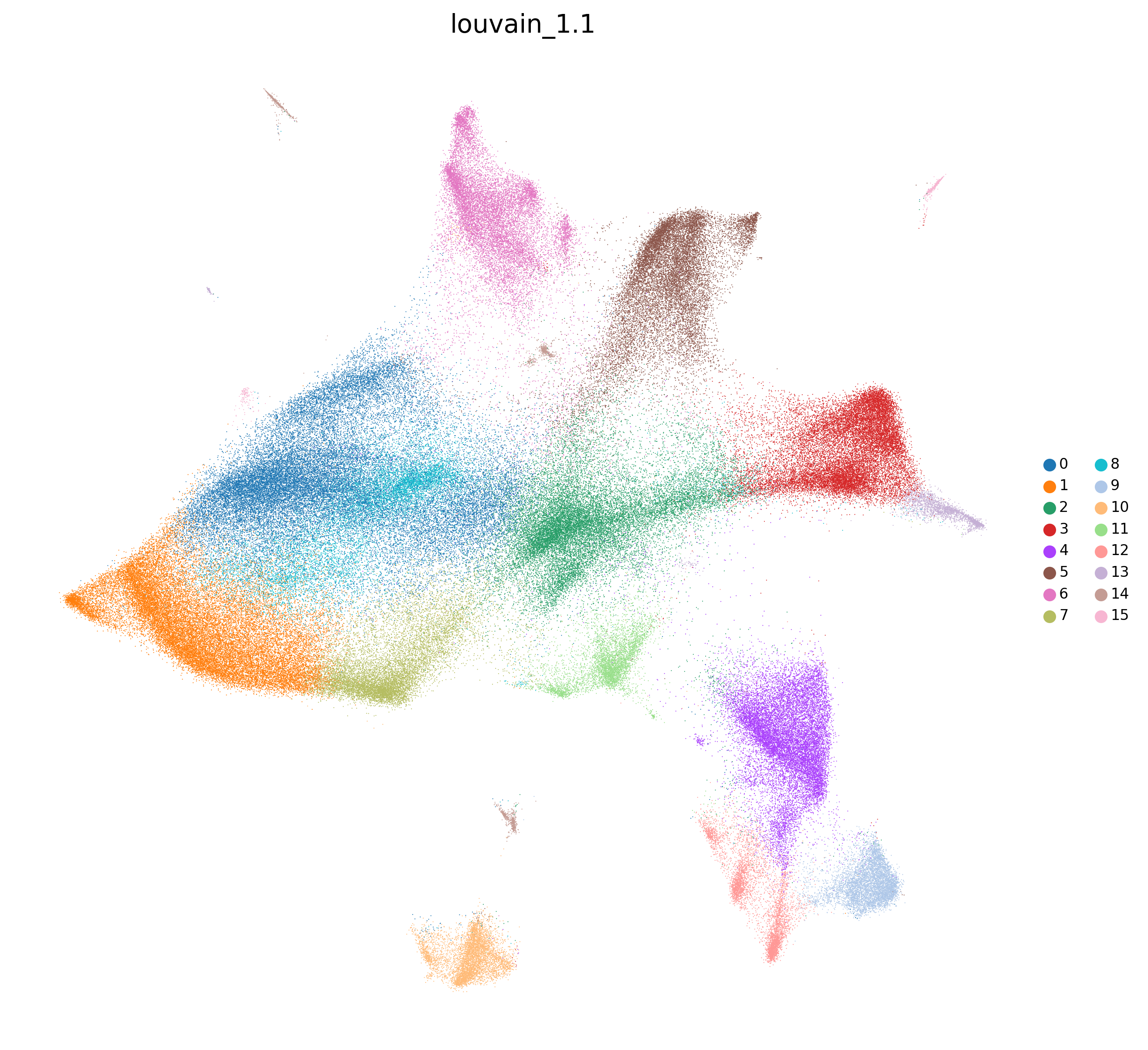
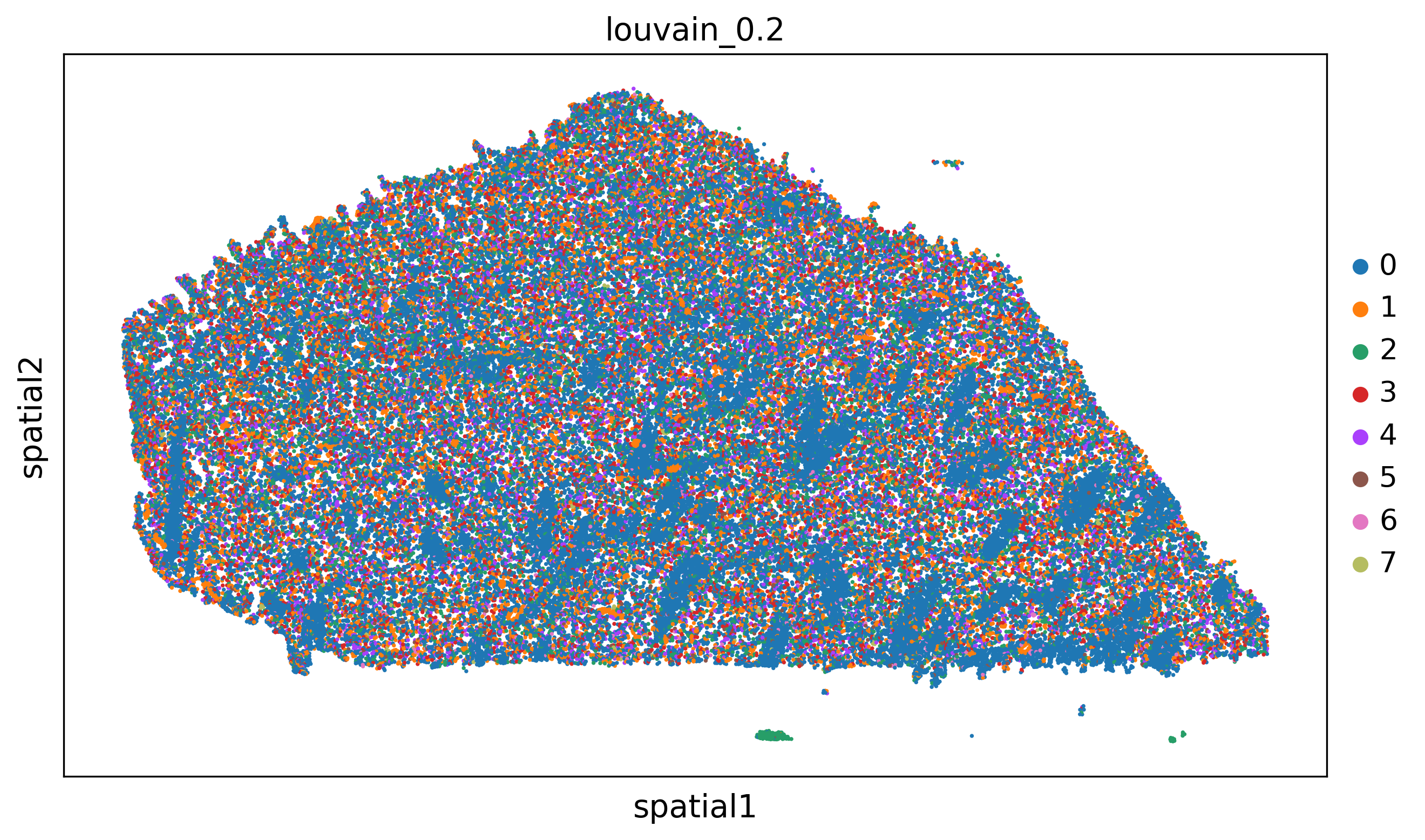
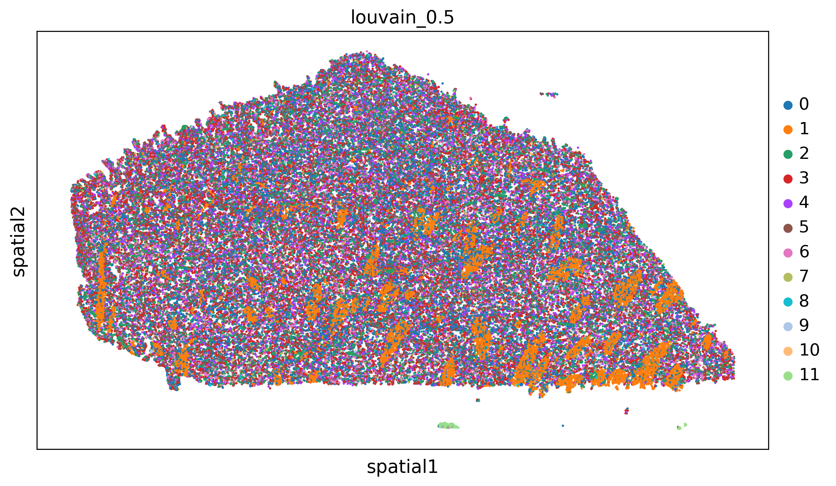
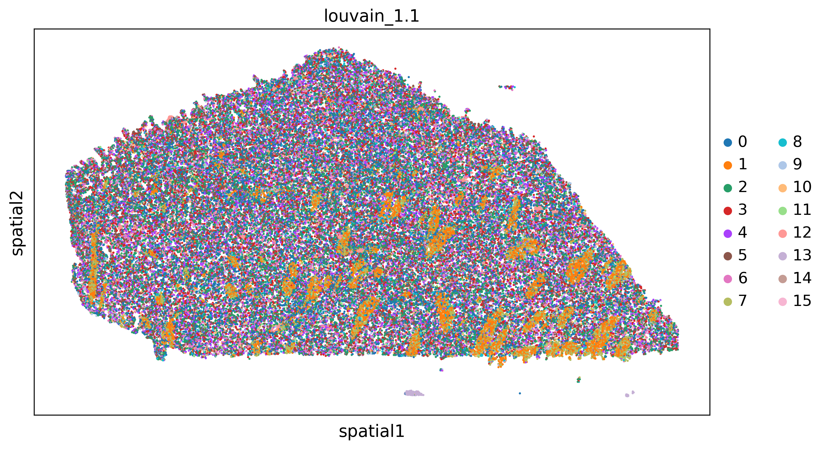
3. Preprocess and cluster cells AnnData
Next we will preprocess cells in our Xenium experiments and cluster them. For this we need to define multiple preprocessing and clustering parameters, present in clustering_params. Within this, we need to define:
normalization_target_sum: Target sum to use if the normalization is done based on library size. None is used for automatic calculation of library size
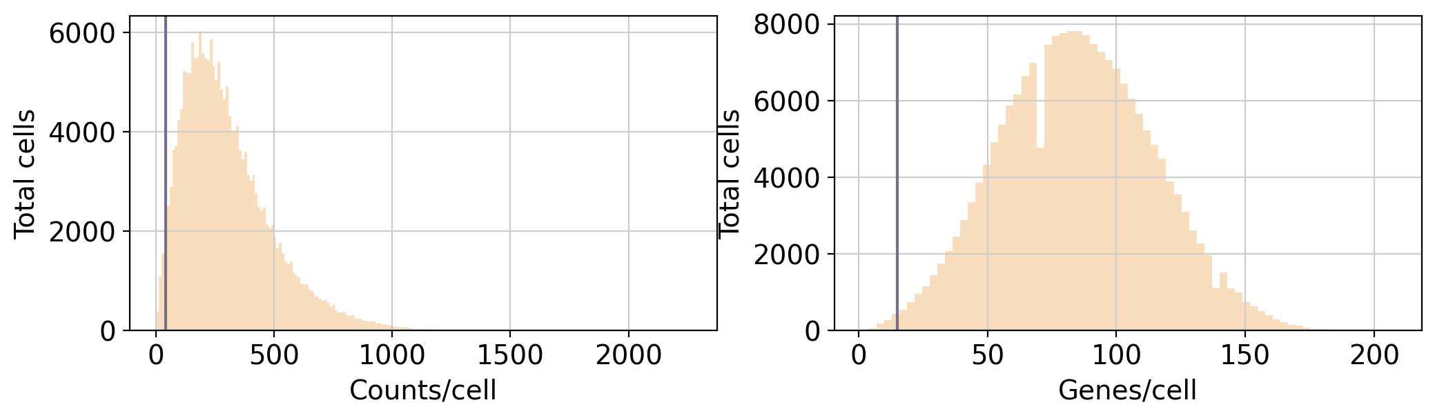
min_counts_x_cell:Minimum amount of counts detected in a cell to pass the quality filters
min_genes_x_cell: Minimum amount of genes expressed in a cell to pass the quality filters
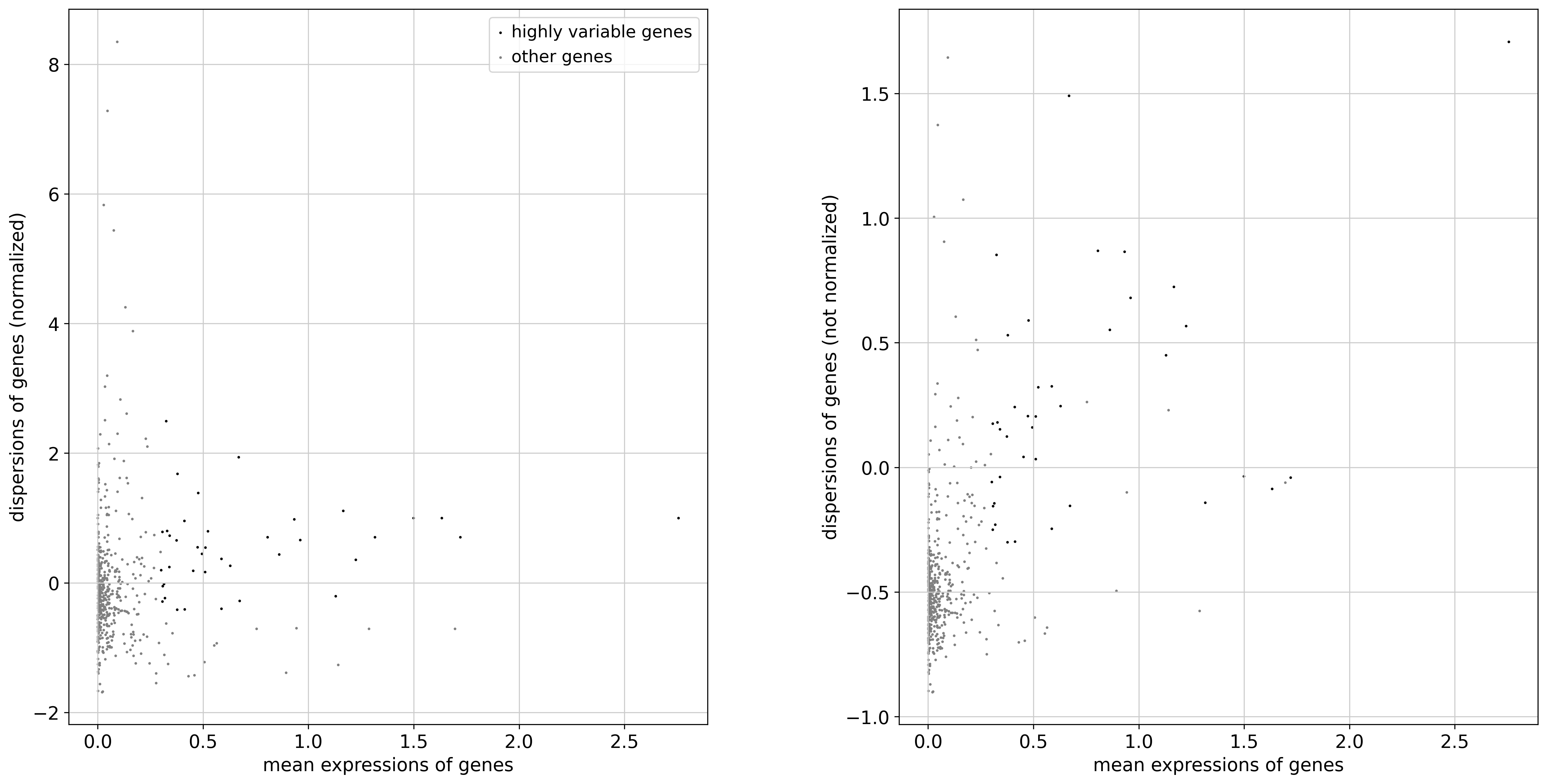
hvg(boolean): whether to select highly variable genes for further processing or not
clustering_alg: which clustering algorithm to use (either louvain or leiden
resolutions: which resolutions to use when clustering
n_neighbors: number of neighbors to used when calculating the nearest neighbors by sc.pp.neighbors()
umap_min_dist: minimum distance when computing UMAP
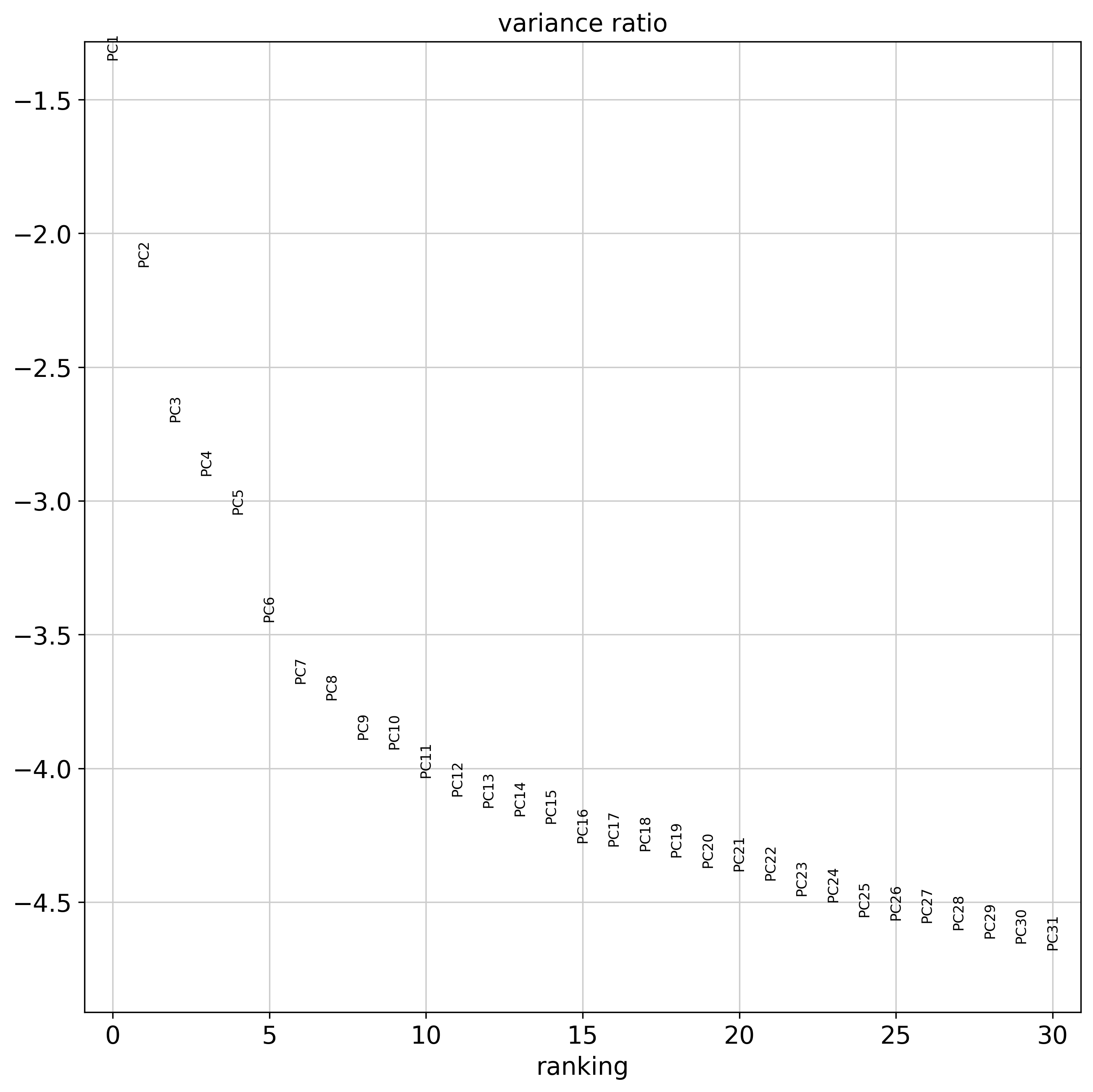
n_pcs: number of principal components to used when calculating the nearest neighbors by sc.pp.neighbors()
The default parameters specified in the example correspond to the parameters found to be optimal when defining best practice. However, we always recommend to adjust them to your own convenience.
[7]:
# Formatting filesand preprocessing
clustering_params={'normalization_target_sum':100,
'min_counts_x_cell':40,
'min_genes_x_cell':15,
'scale':False,
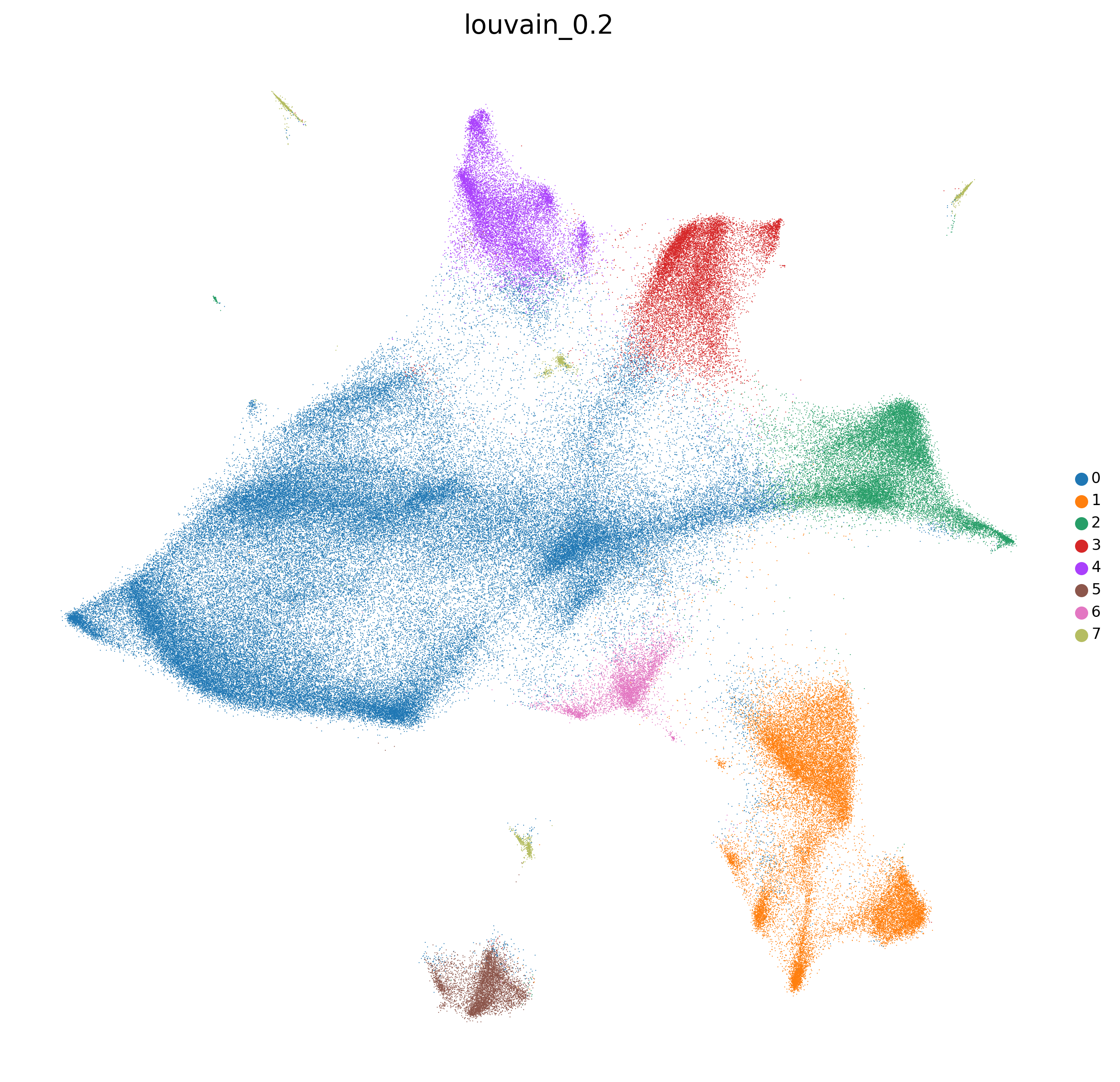
'clustering_alg':'louvain',
'resolutions':[0.2,0.5,1.1],
'n_neighbors':15,'umap_min_dist':0.1,
'n_pcs':0}
[OPTIONAL] Read again the data
[3]:
adata=sc.read(output_path+'combined_filtered.h5ad')
Preprocess adata using predefined parameters
[8]:
adata=preprocess_adata(adata,save=True,clustering_params=clustering_params,output_path=output_path)
/home/sergio/anaconda3/envs/xb_dev3/lib/python3.7/site-packages/anndata/_core/anndata.py:1828: UserWarning: Observation names are not unique. To make them unique, call `.obs_names_make_unique`.
  utils.warn_names_duplicates("obs")
WARNING: It seems you use rank_genes_groups on the raw count data. Please logarithmize your data before calling rank_genes_groups.
WARNING: It seems you use rank_genes_groups on the raw count data. Please logarithmize your data before calling rank_genes_groups.
WARNING: It seems you use rank_genes_groups on the raw count data. Please logarithmize your data before calling rank_genes_groups.
<Figure size 1500x1500 with 0 Axes>
<Figure size 1500x1500 with 0 Axes>
<Figure size 1500x1500 with 0 Axes>
<Figure size 1500x1500 with 0 Axes>
<Figure size 1500x1500 with 0 Axes>
<Figure size 1500x1500 with 0 Axes>
4. Domain identification (use any of the following algorithms in 4.1-3)
4.1 Banksy’s domain identification
[OPTIONAL] Read again the data
[9]:
adata=sc.read(output_path+'combined_processed.h5ad')
/home/sergio/anaconda3/envs/xb_dev3/lib/python3.7/site-packages/anndata/_core/anndata.py:1828: UserWarning: Observation names are not unique. To make them unique, call `.obs_names_make_unique`.
  utils.warn_names_duplicates("obs")
Import required packages
[11]:
from xb.domain_identification import *
import random
random_seed = 1234
np.random.seed(random_seed)
We first define Bansky’s hyperparameters. In summary, this is what they are: - resolutions: clustering resolutions for clustering - cluster_algorithm: clustering algorithm to use in the definition of domain (‘leiden,’louvain’) - pca_dims: number of principal components used to identify the domains in situ - lambda_list: lambda’s parameters to be used when identifying domain. This is, in proportion, how much do you rely on the expression of each cell vs its neighbors. Values close to 1 are used for relying on the expression of neighboring cells (for domain identifications). Values close to 0 are used for regular clustering with little to no influence of neighboring cells - k_geom: number of spatial neighbors of each cell to consider in the definition of each cell based on neighboring cells - max_m’: indicates whether to use the AGF (max_m = 1) or just the mean expression (max_m = 0). By default, we set max_m = 1. - nbr_weight_decay’ : how we assign weights (dependent on inter-cell spatial distances) to edges in the connected spatial graph. By default, we use the gaussian decay option, where weights decay as a function of distnace to the index cell with = sigma. As default, we set to be the median distance between cells, and do not prescribe any cutoff-radius p_outside (no cutoff is conducted).
Please refer to Banksy’s original publication Singhal et al. 2024
[12]:
'''Input File'''
banksy_params={'resolutions':[.9], # clustering resolution for Leiden clustering
'pca_dims':[20], # number of dimensions to keep after PCA
'lambda_list':[.8],# lambda
'k_geom':15, # 15 spatial neighbours
'max_m':1, # use AGF
'nbr_weight_decay':"scaled_gaussian", # can also be "reciprocal", "uniform" or "ranked"
'cluster_algorithm':'leiden'}
Run Banksy
[13]:
adata,adata_banksy=domains_by_banksy(adata,plot_path=plot_path,banksy_params=banksy_params,save=save)
Median distance to closest cell = 15.106551607756607
---- Ran median_dist_to_nearest_neighbour in 0.64 s ----
---- Ran generate_spatial_distance_graph in 1.38 s ----
---- Ran row_normalize in 1.15 s ----
---- Ran generate_spatial_weights_fixed_nbrs in 9.31 s ----
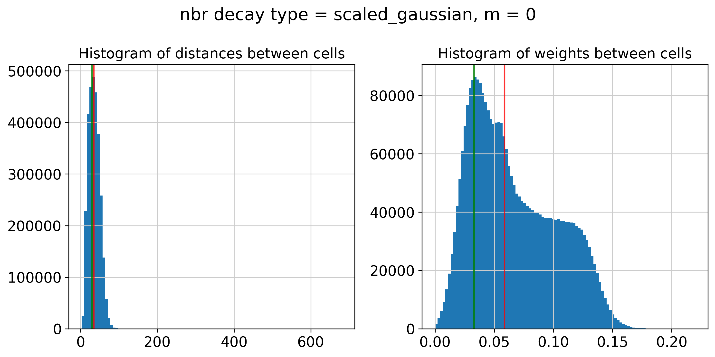
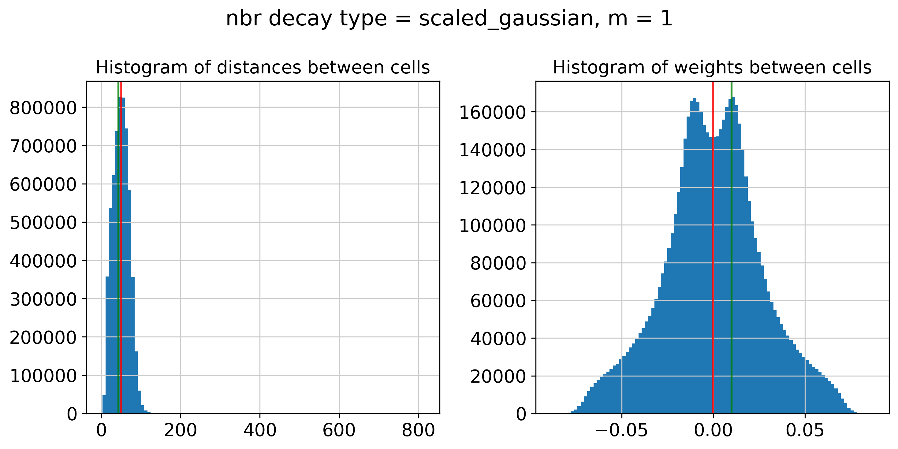
----- Plotting Edge Histograms for m = 0 -----
Edge weights (distances between cells): median = 34.56489338313938, mode = 29.92653359499485
---- Ran plot_edge_histogram in 0.14 s ----
Edge weights (weights between cells): median = 0.05877572185687528, mode = 0.032933527590574184
---- Ran plot_edge_histogram in 0.14 s ----
---- Ran generate_spatial_distance_graph in 2.14 s ----
---- Ran theta_from_spatial_graph in 2.18 s ----
---- Ran row_normalize in 1.16 s ----
---- Ran generate_spatial_weights_fixed_nbrs in 12.57 s ----
----- Plotting Edge Histograms for m = 1 -----
Edge weights (distances between cells): median = 49.69937497424205, mode = 43.32784977890054
---- Ran plot_edge_histogram in 0.21 s ----
Edge weights (weights between cells): median = (1.3453800709411726e-05+0.004469004013761351j), mode = (0.010014964691843362+0.00368228208036008j)
---- Ran plot_edge_histogram in 0.52 s ----
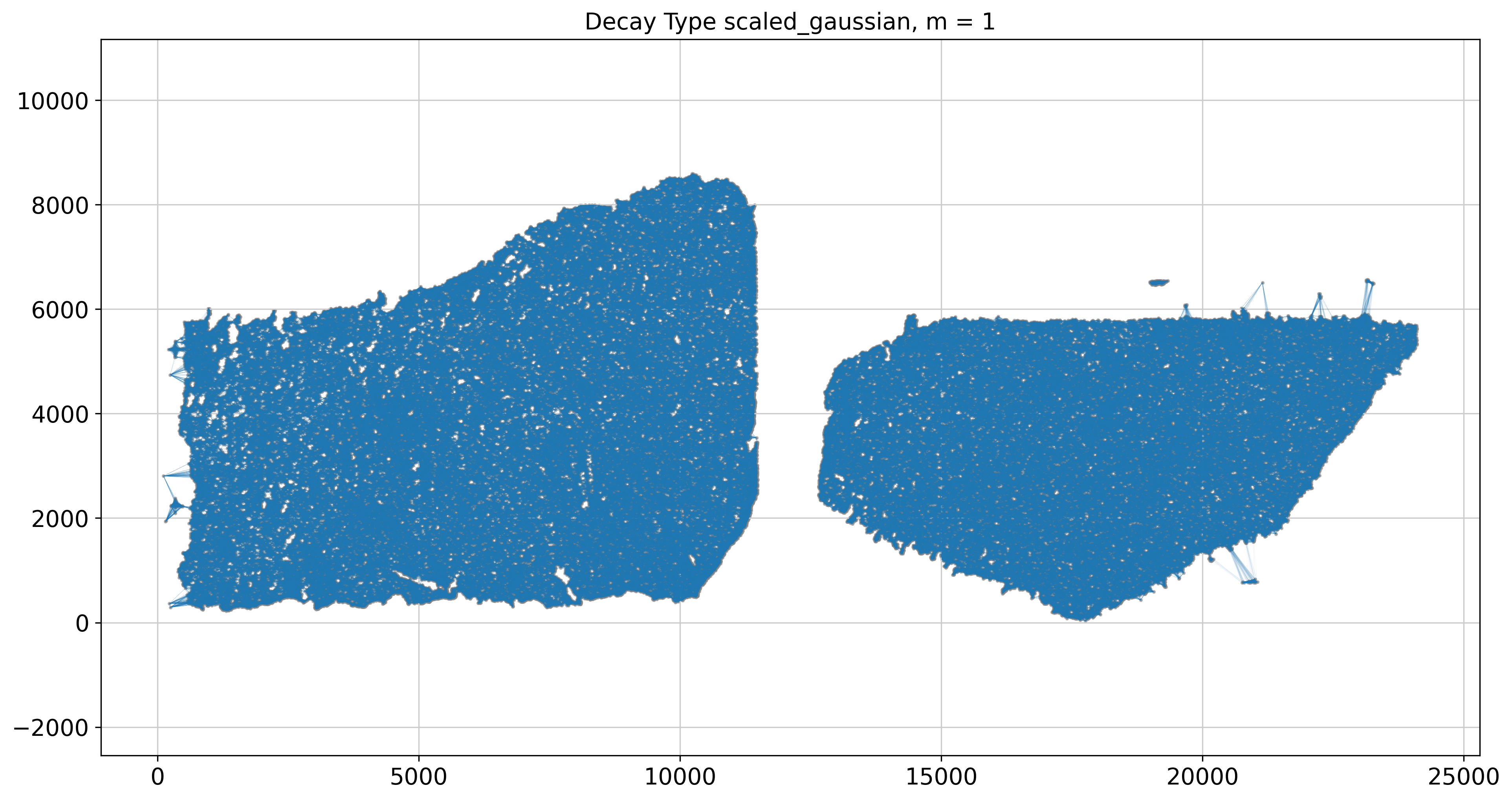
----- Plotting Weights Graph -----
Maximum weight: 0.21955685060382787
---- Ran plot_graph_weights in 34.85 s ----
Maximum weight: (0.08713431717306296-0.0012601695417479744j)
---- Ran plot_graph_weights in 65.41 s ----
Runtime Jun-14-2024-12-18
541 genes to be analysed:
Gene List:
Index(['ABCC4', 'ABCC9', 'ACTN2', 'ADAMTS12', 'ADAMTS16', 'ADAMTS3', 'ADRA1A',
'ADRA1B', 'AIF1', 'ALK',
...
'BLANK_0376', 'BLANK_0381', 'BLANK_0393', 'DeprecatedCodeword_0160',
'DeprecatedCodeword_0171', 'DeprecatedCodeword_0196',
'DeprecatedCodeword_0304', 'DeprecatedCodeword_0318',
'DeprecatedCodeword_0344', 'DeprecatedCodeword_0373'],
dtype='object', name='gene_id', length=541)
Decay Type: scaled_gaussian
Weights Object: {'weights': {0: <196570x196570 sparse matrix of type '<class 'numpy.float64'>'
with 2948550 stored elements in Compressed Sparse Row format>, 1: <196570x196570 sparse matrix of type '<class 'numpy.complex128'>'
with 5897100 stored elements in Compressed Sparse Row format>}}
Nbr matrix | Mean: 0.09 | Std: 0.25
Size of Nbr | Shape: (196570, 541)
Top 3 entries of Nbr Mat:
[[0.04155145 0.04730741 0.08066992]
[0.07221414 0.05093029 0.2353539 ]
[0.06404802 0.04749484 0.22760928]]
AGF matrix | Mean: 0.02 | Std: 0.03
Size of AGF mat (m = 1) | Shape: (196570, 541)
Top entries of AGF:
[[0.02035019 0.00812465 0.01449246]
[0.03237184 0.00993546 0.03555132]
[0.0431125 0.00850346 0.02896317]]
Ran 'Create BANKSY Matrix' in 0.78 mins
Cell by gene matrix has shape (196570, 541)
Scale factors squared: [0.2 0.53333333 0.26666667]
Scale factors: [0.4472136 0.73029674 0.51639778]
Shape of BANKSY matrix: (196570, 1623)
Type of banksy_matrix: <class 'anndata._core.anndata.AnnData'>
Current decay types: ['scaled_gaussian']
Reducing dims of dataset in (Index = scaled_gaussian, lambda = 0.8)
==================================================
Setting the total number of PC = 20
Original shape of matrix: (196570, 1623)
Reduced shape of matrix: (196570, 20)
------------------------------------------------------------
min_value = -12.465734481811523, mean = 2.384801973676076e-06, max = 26.507896423339844
Conducting clustering with Leiden Parition
Decay type: scaled_gaussian
Neighbourhood Contribution (Lambda Parameter): 0.8
reduced_pc_20
PCA dims to analyse: [20]
====================================================================================================
Setting up partitioner for (nbr decay = scaled_gaussian), Neighbourhood contribution = 0.8, PCA dimensions = 20)
====================================================================================================
Nearest-neighbour weighted graph (dtype: float64, shape: (196570, 196570)) has 9828500 nonzero entries.
---- Ran find_nn in 2197.69 s ----
Nearest-neighbour connectivity graph (dtype: int16, shape: (196570, 196570)) has 9828500 nonzero entries.
(after computing shared NN)
Allowing nearest neighbours only reduced the number of shared NN from 305511494 to 9785171.
Shared nearest-neighbour (connections only) graph (dtype: int16, shape: (196570, 196570)) has 8231792 nonzero entries.
Shared nearest-neighbour (number of shared neighbours as weights) graph (dtype: int16, shape: (196570, 196570)) has 8231792 nonzero entries.
sNN graph data:
[ 7 9 7 ... 17 17 14]
---- Ran shared_nn in 35.46 s ----
-- Multiplying sNN connectivity by weights --
shared NN with distance-based weights graph (dtype: float64, shape: (196570, 196570)) has 8231792 nonzero entries.
shared NN weighted graph data: [0.17257742 0.17265785 0.17291254 ... 0.29328497 0.33253759 0.42289093]
Converting graph (dtype: float64, shape: (196570, 196570)) has 8231792 nonzero entries.
---- Ran csr_to_igraph in 3.84 s ----
Resolution: 0.9
------------------------------
---- Partitioned BANKSY graph ----
modularity: 0.78
18 unique labels:
[ 0 1 2 3 4 5 6 7 8 9 10 11 12 13 14 15 16 17]
---- Ran partition in 225.39 s ----
Computing ARI for annotated labels
Label Dense [ 1 2 2 ... 17 17 17]
After sorting Dataframe
Shape of dataframe: (1, 8)
| decay | lambda_param | num_pcs | resolution | num_labels | labels | adata | ari | |
|---|---|---|---|---|---|---|---|---|
| scaled_gaussian_pc20_nc0.80_r0.90 | scaled_gaussian | 0.8 | 20 | 0.9 | 18 | Label object:\nNumber of labels: 18, number of... | [[[View of AnnData object with n_obs × n_vars ... | 0.0 |
Anndata AxisArrays with keys: reduced_pc_20

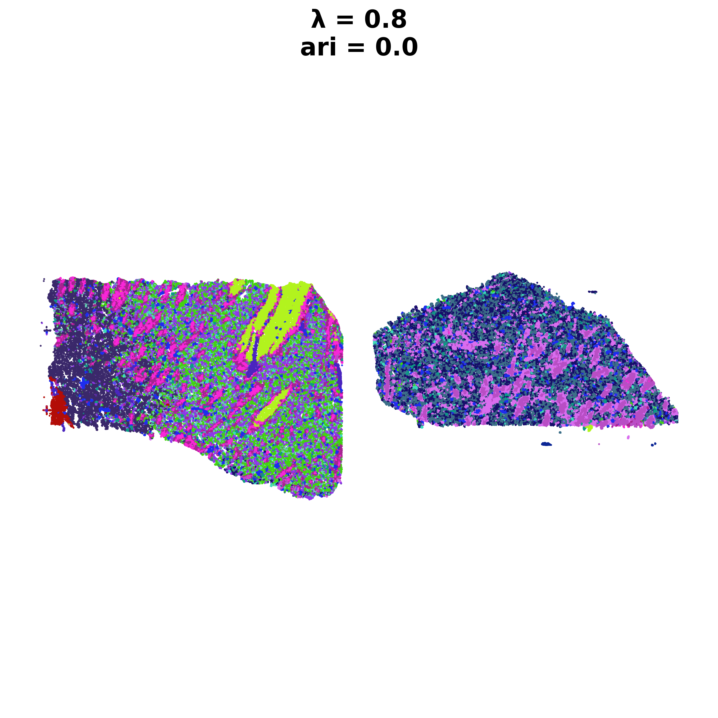
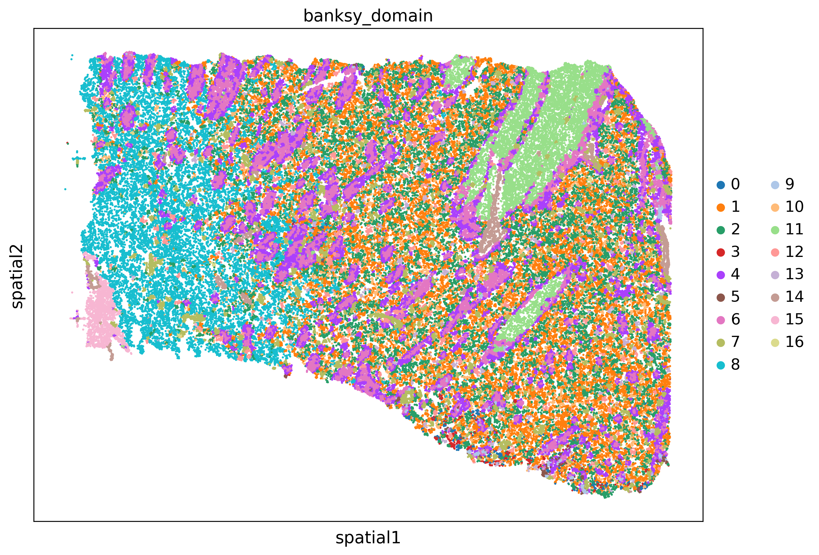
[14]:
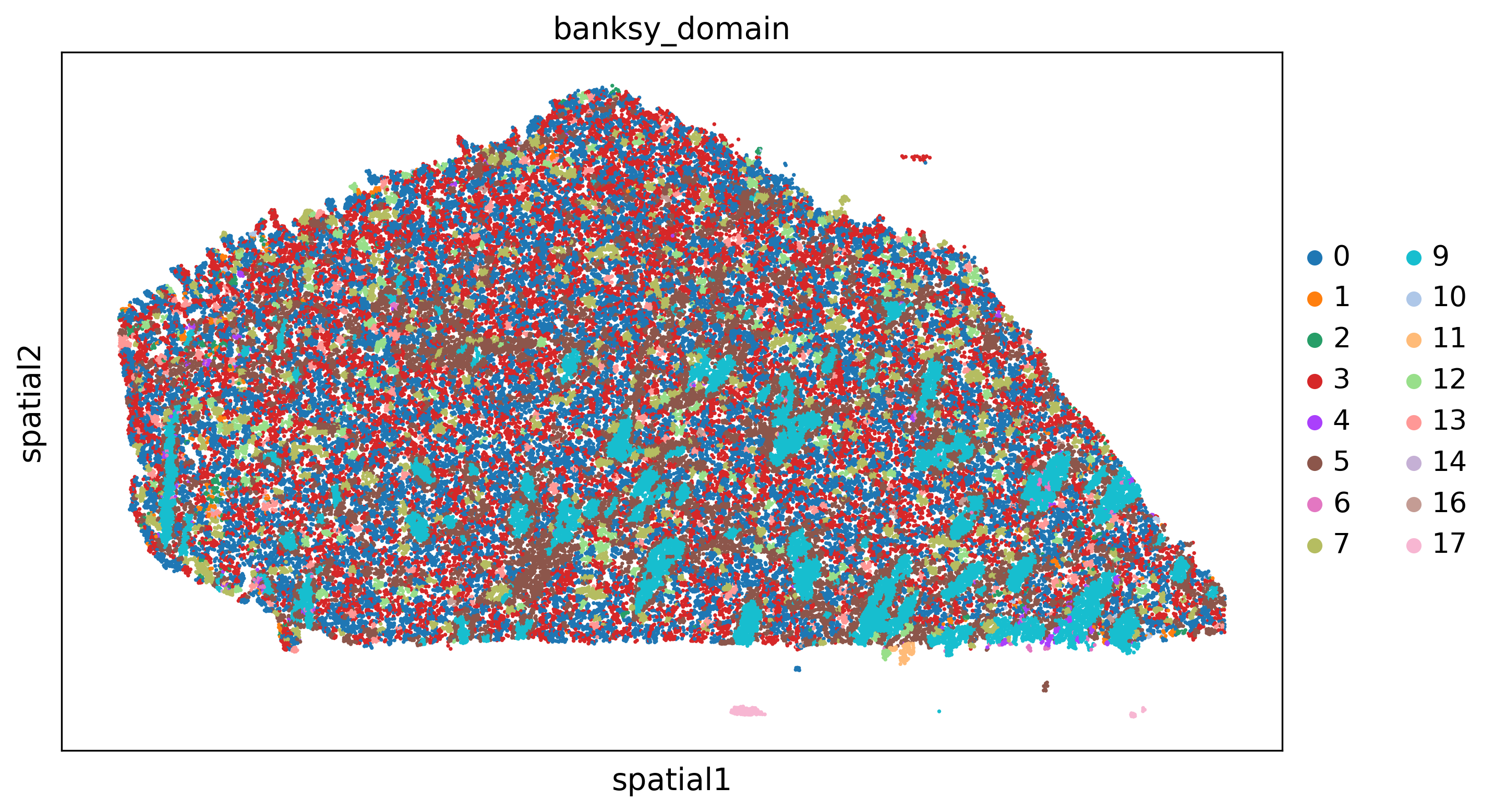
for s in adata.obs['sample'].unique():
        adatasub=adata[adata.obs['sample']==s]
        sc.pl.spatial(adatasub,color='banksy_domain',spot_size=40)
4.2 Neighbors-based domain identification (NBD)
[15]:
from xb.formatting import format_data_neighs
hyperparameters_nbd={'key':'louvain_1.1','resolution':1.0,'neighbors':15,'clustering_algorithm':'leiden'}
[16]:
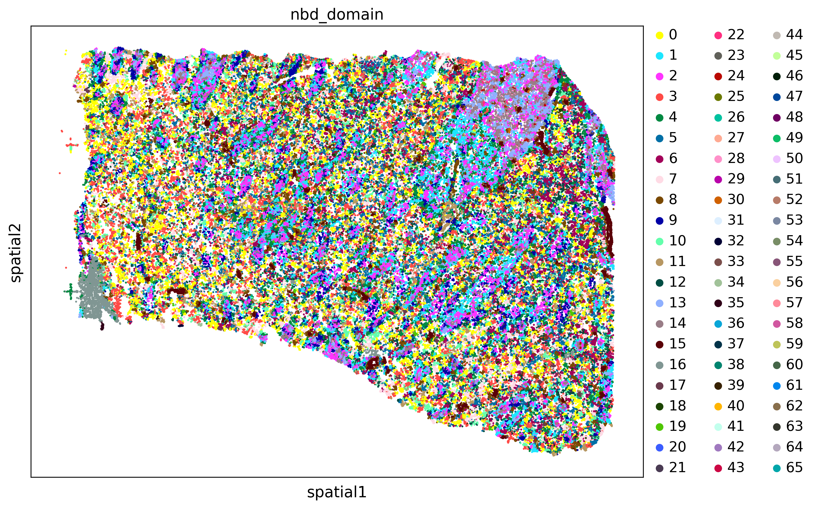
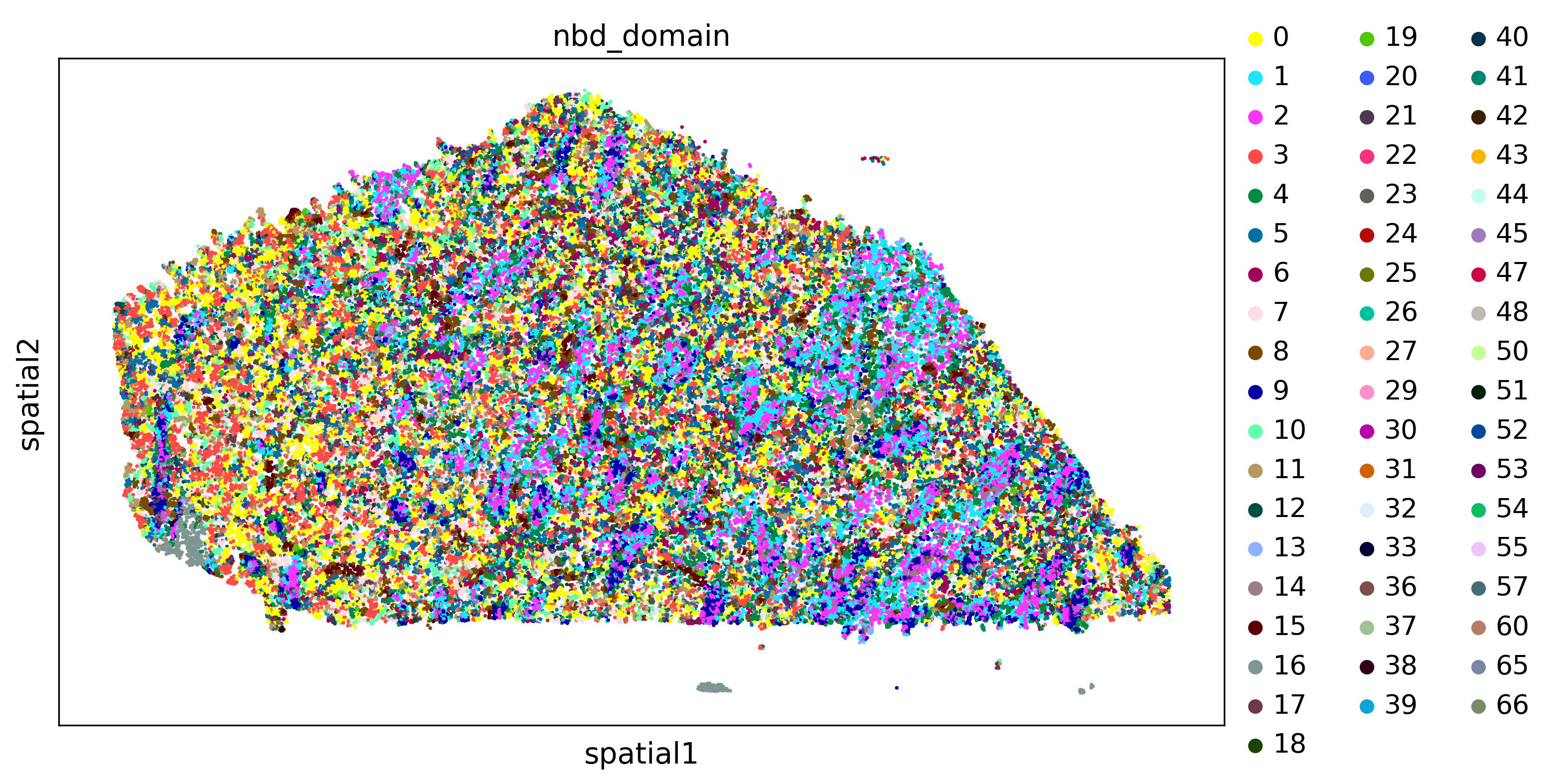
adata,adata_nbd=domains_by_nbd(adata,hyperparameters_nbd=hyperparameters_nbd)
100%|███████████████████████████████████████████████████████████████████████████████████| 16/16 [00:00<00:00, 28.37it/s]
100%|███████████████████████████████████████████████████████████████████████████████████| 16/16 [00:00<00:00, 28.44it/s]
[17]:
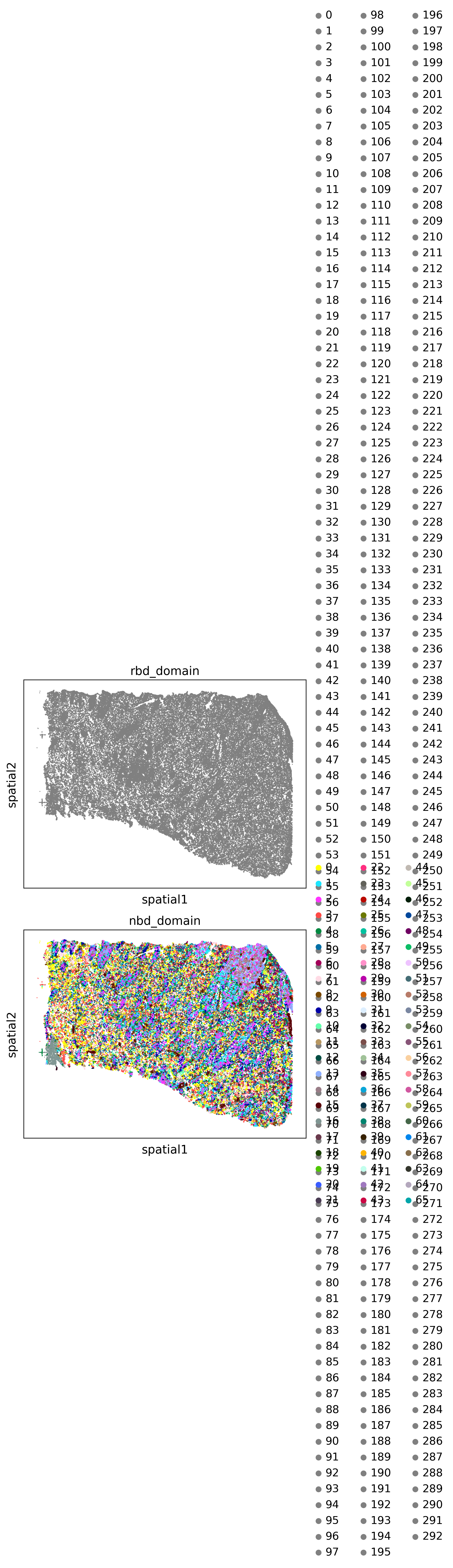
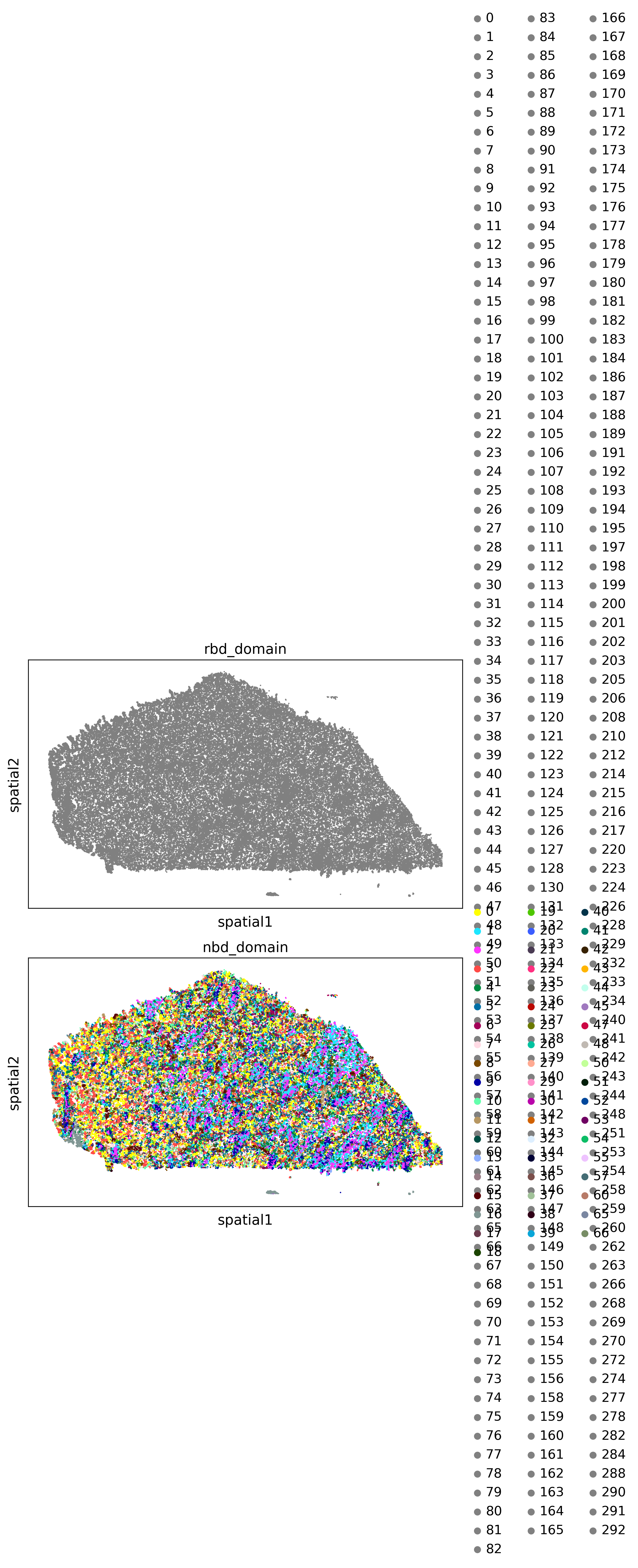
plot_domains(adata,groupby='nbd_domain')
4.3 Read-based domains identification (RBD)
[18]:
hyperparameters_rbd={'key':'louvain_1.1','resolution':0.2,'neighbors':15,'clustering_algorithm':'leiden'}
[19]:
adata,adata_nbd=domains_by_rbd(adata,hyperparameters_rbd=hyperparameters_rbd)
100%|███████████████████████████████████████████████████████████████████████████| 196570/196570 [38:28<00:00, 85.15it/s]
100%|███████████████████████████████████████████████████████████████████████████| 196570/196570 [38:10<00:00, 85.83it/s]
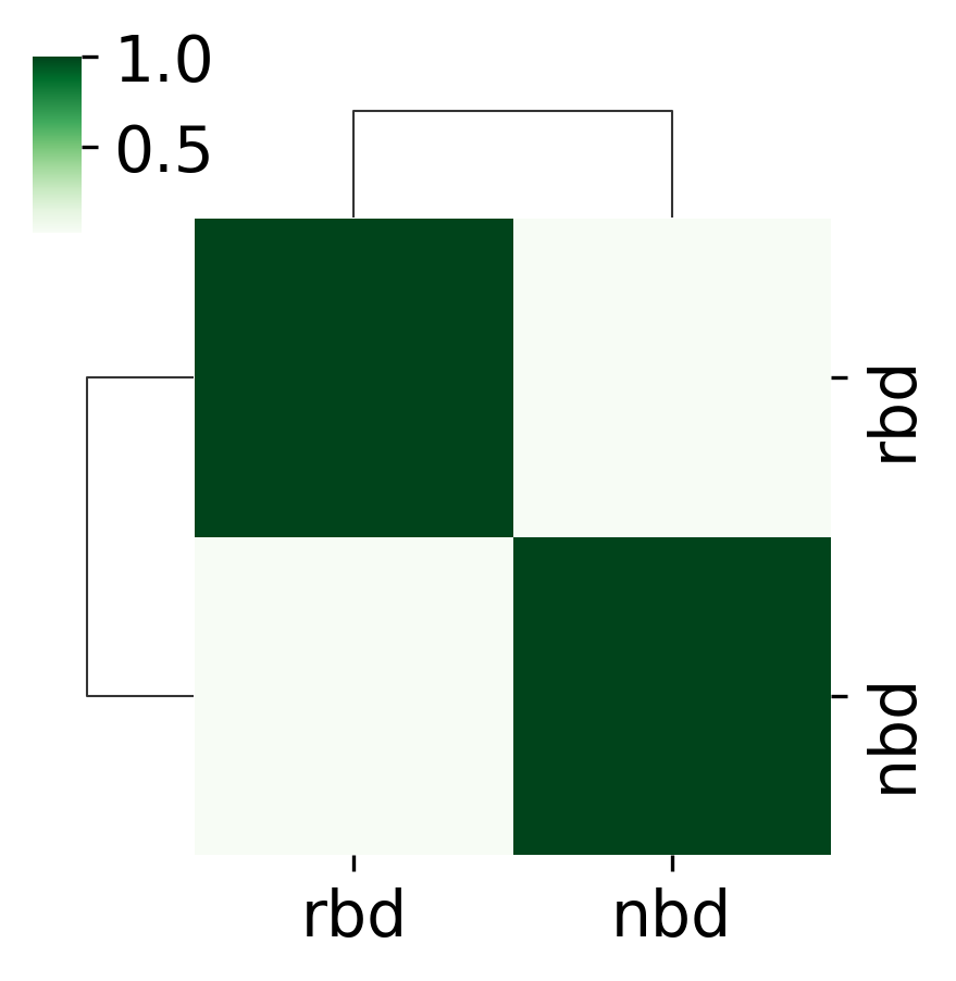
4.4 Compare domains identified by different algorithms
[20]:
domain_keys=['rbd_domain','nbd_domain']#banksy_domain
ARI=compare_domains(adata,domain_keys=domain_keys,plot_path=plot_path,save=True)
<Figure size 1500x1500 with 0 Axes>
5 Imputation using SpaGE
[21]:
import numpy as np
import pandas as pd
import matplotlib.pyplot as plt
import scipy.stats as st
import warnings
from xb.Spage_main import * #make sure this works
Please specify where the single cell data in the format of h5ad is stored
[22]:
adata_sc=sc.read('./data/data_end_to_end_pipeline/scRNAseq.h5ad')
[27]:
adata_sc.X=adata_sc.X.todense()
adata_sc.X=adata_sc.X.astype('float64')
adata.X=adata.X.astype('float64')
adata=adata[:,adata.var.index.isin(adata_sc.var.index)]
[ ]:
Imp_genes=leave_one_out_validation(adata,adata_sc,genes=['DRD1','DRD2'])
[49]:
new_genes = ['DRD1','DRD2']
Imp_New_Genes=gene_imputation(adata,adata_sc,new_genes)
6.Identifying Spatially variabile genes (SVF) by Squidpy’s Moran I
[61]:
adata,hs_results=svf_moranI(adata,radius=50.0)
[62]:
hs_results.head(10)
[62]:
| Pval | FDR | rank | |
|---|---|---|---|
| EFHD1 | 0.0 | 0.0 | 364.0 |
| THBS1 | 0.0 | 0.0 | 363.0 |
| FCGR3A | 0.0 | 0.0 | 362.0 |
| MOBP | 0.0 | 0.0 | 361.0 |
| IGFBP4 | 0.0 | 0.0 | 360.0 |
| ATP5F1E | 0.0 | 0.0 | 359.0 |
| GAPDH | 0.0 | 0.0 | 358.0 |
| CRYAB | 0.0 | 0.0 | 357.0 |
| ERMN | 0.0 | 0.0 | 356.0 |
| DBNDD2 | 0.0 | 0.0 | 355.0 |
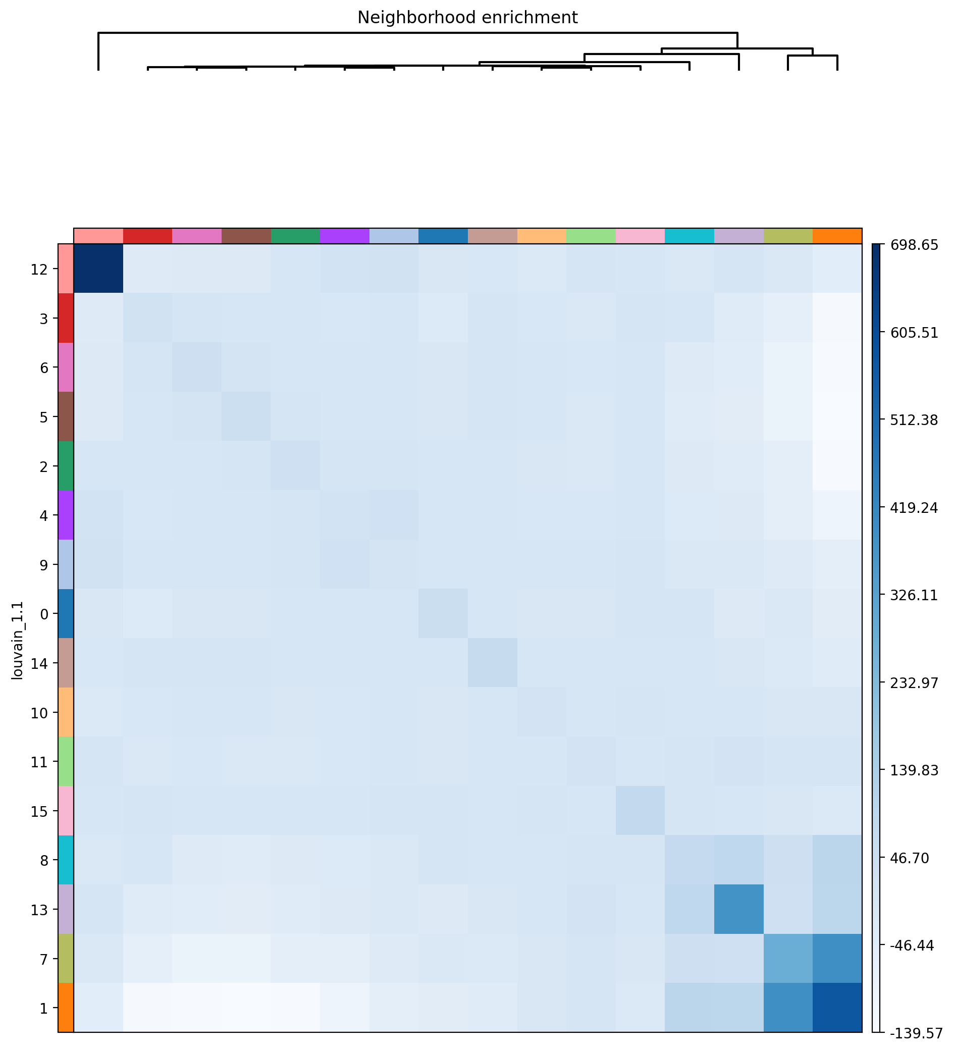
7. Defining neighborhood enrichment of celltypes using Squidpy
[54]:
from xb.neighborhood import *
[55]:
adata=nhood_squidpy(adata,sample_key='sample',radius=50.0,cluster_key='louvain_1.1',plot_path=plot_path,cmap='Blues')
[ ]: